In Session 2, we used linear regression to model a continuous outcome (distance to school) and introduced the Linear Probability Model (LPM) as a simple way to handle binary outcomes. In this session, we go further with the proper tool for binary outcomes: logistic regression.
We need to load the packages and data as before, and to create a survey design object:
# Load necessary packagesload.lib <-c("tidyverse", "survey", "srvyr","gtsummary","performance","ggstats","broom.helpers","marginaleffects")install.lib <- load.lib[!load.lib %in%installed.packages()]for (lib in install.lib) install.packages(lib, dependencies =TRUE)sapply(load.lib, require, character =TRUE)
About 29% of children walk to school (svymean(~walk, design_edu, na.rm = TRUE)), making it a well-suited outcome for logistic regression.
By the end of this session, you will be able to:
Understand whether logistic regression is preferable to the LPM for binary outcomes
Estimate a logistic regression model on weighted survey data
Interpret log-odds, odds ratios, and predicted probabilities
Present results in publication-ready tables and figures
Compare LPM and logistic regression results
11.1 Why Logistic Regression?
Recall from Session 2 that the LPM applies linear regression directly to a binary outcome. Its main limitation is that predicted values can fall outside [0, 1] — which is theoretically incoherent for a probability.
Logistic regression solves this by modelling the log-odds of the outcome, using a logistic transformation to keep all predicted probabilities between 0 and 1:
The trade-off is that coefficients are on the log-odds scale, which is less directly interpretable than the LPM’s percentage point differences — but we will see how to convert them into more intuitive quantities.
11.2 Estimating the Model
With weighted survey data, we use svyglm() with family = quasibinomial():
model_logit <-svyglm( walk ~ sex + age + edu_parent + hhwealthcat + province,design = design_edu,family =quasibinomial())summary(model_logit)
Call:
svyglm(formula = walk ~ sex + age + edu_parent + hhwealthcat +
    province, design = design_edu, family = quasibinomial())

Survey design:
Called via srvyr

Coefficients:
                           Estimate Std. Error t value Pr(>|t|)
(Intercept)                 0.55354    0.30233   1.831 0.067205 .
sexFemale                  -0.01417    0.08871  -0.160 0.873056
age                        -0.03395    0.01165  -2.913 0.003601 **
edu_parentPrimary          -0.05279    0.25539  -0.207 0.836241
edu_parentJunior secondary -0.36598    0.23743  -1.541 0.123313
edu_parentSenior secondary -0.54647    0.24845  -2.199 0.027915 *
edu_parentCollegiate       -0.74053    0.26762  -2.767 0.005688 **
edu_parentTertiary         -0.88338    0.36467  -2.422 0.015474 *
hhwealthcatPoor            -0.56425    0.13042  -4.326 1.56e-05 ***
hhwealthcatMiddle          -0.65508    0.13972  -4.689 2.86e-06 ***
hhwealthcatRich            -0.98726    0.14794  -6.674 2.93e-11 ***
hhwealthcatRichest         -1.77988    0.20025  -8.888  < 2e-16 ***
provinceCentral             0.55647    0.15130   3.678 0.000239 ***
provinceSouthern            0.01338    0.15684   0.085 0.932013
provinceNorthern           -0.26094    0.17227  -1.515 0.129950
provinceEastern             0.96948    0.15470   6.267 4.18e-10 ***
provinceNorth Western      -0.57639    0.19108  -3.016 0.002577 **
provinceNorth Central      -0.43617    0.23087  -1.889 0.058948 .
provinceUva                 0.24346    0.19318   1.260 0.207657
provinceSabaragamuwa        0.13064    0.20220   0.646 0.518257
---
Signif. codes:  0 '***' 0.001 '**' 0.01 '*' 0.05 '.' 0.1 ' ' 1

(Dispersion parameter for quasibinomial family taken to be 0.9868737)

Number of Fisher Scoring iterations: 4
Why quasibinomial and not binomial?
With survey data, observations are not independent. Using quasibinomial() avoids the assumption of binomial variance and produces correct standard errors for weighted data. The point estimates (coefficients) are identical to binomial().
11.3 Interpreting Coefficients: Odds Ratios
The raw coefficients are on the log-odds scale, which is not intuitive. We exponentiate them to obtain odds ratios (OR):
tbl_regression(model_logit, exponentiate =TRUE)
Characteristic
OR
95% CI
p-value
sex
Male
—
—
Female
0.99
0.83, 1.17
0.9
age
0.97
0.94, 0.99
0.004
Educational attainment
Less than primary
—
—
Primary
0.95
0.57, 1.57
0.8
Junior secondary
0.69
0.44, 1.10
0.12
Senior secondary
0.58
0.36, 0.94
0.028
Collegiate
0.48
0.28, 0.81
0.006
Tertiary
0.41
0.20, 0.85
0.015
hhwealthcat
Poorest
—
—
Poor
0.57
0.44, 0.73
<0.001
Middle
0.52
0.39, 0.68
<0.001
Rich
0.37
0.28, 0.50
<0.001
Richest
0.17
0.11, 0.25
<0.001
province
Western
—
—
Central
1.74
1.30, 2.35
<0.001
Southern
1.01
0.75, 1.38
>0.9
Northern
0.77
0.55, 1.08
0.13
Eastern
2.64
1.95, 3.57
<0.001
North Western
0.56
0.39, 0.82
0.003
North Central
0.65
0.41, 1.02
0.059
Uva
1.28
0.87, 1.86
0.2
Sabaragamuwa
1.14
0.77, 1.69
0.5
Abbreviations: CI = Confidence Interval, OR = Odds Ratio
11.3.1 Interpreting an odds ratio
OR = 1: no association with the outcome
OR > 1: this category is more likely to walk to school
OR < 1: this category is less likely to walk to school
For example, an OR of 0.17 for hhwealthcatRichest means children from the richest households have 6 times lower odds of walking to school compared to the poorest (1/0.17 ≈ 6) — consistent with wealthier families being more likely to use motorised transport. We can also say that children from the richest households have 83% lower odds of walking to school compared to the poorest [(1 - 0.17) × 100 = 83%].
Or we can also say from the results that children from the Central province have 1.74 times higher odds of walking to school compared to children from the Western province.
Odds ratios vs. percentage point differences
Odds ratios describe relative effects and can be counterintuitive, especially when the outcome is common. An OR of 0.5 does not mean the probability is halved — the actual difference in probability depends on the baseline probability. For a more direct interpretation, see the note on marginal effects at the end of this session.
Odds Ratios below 1 are less intuitive to understand and grasp. It may be useful to change the reference category of the variable of interest to get ORs > 1!
11.4 Nested Model Comparison
As in Session 2, we compare nested models to assess the contribution of each block of variables:
m1 <-svyglm(walk ~ sex + age, design = design_edu, family =quasibinomial())m2 <-svyglm(walk ~ sex + age + edu_parent + hhwealthcat, design = design_edu, family =quasibinomial())m3 <-svyglm(walk ~ sex + age + edu_parent + hhwealthcat + province, design = design_edu, family =quasibinomial())tbl_merge(list(tbl_regression(m1, exponentiate =TRUE),tbl_regression(m2, exponentiate =TRUE),tbl_regression(m3, exponentiate =TRUE) ),tab_spanner =c("Model 1", "Model 2", "Model 3"))
Characteristic
Model 1
Model 2
Model 3
OR
95% CI
p-value
OR
95% CI
p-value
OR
95% CI
p-value
sex
Male
—
—
—
—
—
—
Female
0.98
0.84, 1.13
0.7
0.97
0.82, 1.15
0.8
0.99
0.83, 1.17
0.9
age
0.98
0.96, 1.00
0.035
0.97
0.95, 0.99
0.004
0.97
0.94, 0.99
0.004
Educational attainment
Less than primary
—
—
—
—
Primary
1.00
0.62, 1.60
>0.9
0.95
0.57, 1.57
0.8
Junior secondary
0.64
0.41, 1.00
0.048
0.69
0.44, 1.10
0.12
Senior secondary
0.57
0.36, 0.90
0.015
0.58
0.36, 0.94
0.028
Collegiate
0.47
0.28, 0.77
0.003
0.48
0.28, 0.81
0.006
Tertiary
0.45
0.23, 0.91
0.026
0.41
0.20, 0.85
0.015
hhwealthcat
Poorest
—
—
—
—
Poor
0.57
0.44, 0.72
<0.001
0.57
0.44, 0.73
<0.001
Middle
0.48
0.37, 0.63
<0.001
0.52
0.39, 0.68
<0.001
Rich
0.35
0.27, 0.46
<0.001
0.37
0.28, 0.50
<0.001
Richest
0.14
0.10, 0.21
<0.001
0.17
0.11, 0.25
<0.001
province
Western
—
—
Central
1.74
1.30, 2.35
<0.001
Southern
1.01
0.75, 1.38
>0.9
Northern
0.77
0.55, 1.08
0.13
Eastern
2.64
1.95, 3.57
<0.001
North Western
0.56
0.39, 0.82
0.003
North Central
0.65
0.41, 1.02
0.059
Uva
1.28
0.87, 1.86
0.2
Sabaragamuwa
1.14
0.77, 1.69
0.5
Abbreviations: CI = Confidence Interval, OR = Odds Ratio
11.4.1 Goodness of fit
The results confirm the pattern observed in Session 2 with linear regression. Model 1, with only sex and age, fits the data very poorly (R² ≈ 0.001) — individual characteristics alone tell us almost nothing about who walks to school. The addition of socioeconomic variables in Model 2 produces a substantial improvement (AIC drops from 4725 to 3546, R² rises to 0.08), confirming that household wealth and parental education are the main drivers of transport mode. Adding province in Model 3 brings a further modest gain (AIC = 3447, R² = 0.11), suggesting that geographic context plays an additional but secondary role — consistent with the linear regression findings in Session 2.
Note
Lower AIC indicates better fit, penalising model complexity. The R² reported here is a survey-adapted approximation (correlation between fitted values and observed outcome, squared), comparable to the one used in Session 2. For logistic regression, it should be interpreted cautiously — what matters most for model comparison is the AIC.
# Comparison of Model Performance Indices

Name |  Model |  AIC (weights) |    R2 | R2 (adj.)
--------------------------------------------------
m1   | svyglm | 4725.1 (<.001) | 0.001 | 5.462e-04
m2   | svyglm | 3546.0 (<.001) | 0.079 |     0.076
m3   | svyglm | 3447.3 (>.999) | 0.109 |     0.104
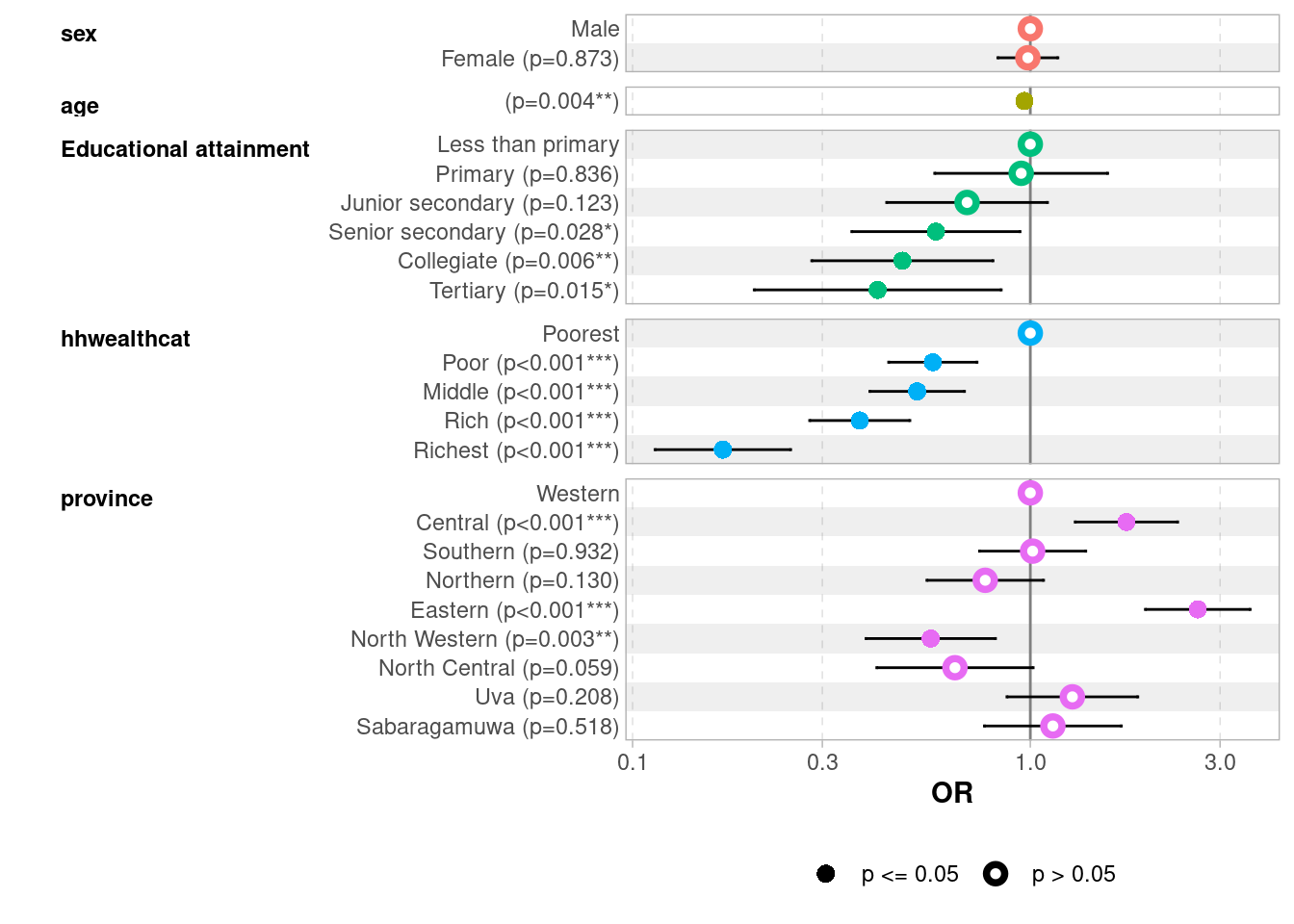
11.5 Visualising Results: A Forest Plot
m3 |> ggstats::ggcoef_model(exponentiate =TRUE)
11.6 LPM vs. Logistic Regression: A Comparison
It is instructive to compare the LPM and logistic regression on the same outcome. In many cases, the two approaches give very similar substantive conclusions.
Here, in both cases, household wealth is the strongest predictor of walking to school, with a clear gradient from poorest to richest; parental education shows a significant negative effect only from Senior secondary upward; and province plays an important role, with Eastern province children being much more likely to walk (OR = 2.64, +22 percentage points) and North Western children much less so.
The LPM coefficients offer a more direct interpretation — for instance, children from the richest households walk to school 31 percentage points less often than the poorest — while logistic regression ensures predicted probabilities remain within [0, 1] (as is verified by computing the marginal predictions from the logistic model).
Abbreviations: CI = Confidence Interval, OR = Odds Ratio
#we have removed the calculation of a marginal prediction for age as it is a continuous#variable.
When results are consistent across both models, it strengthens confidence in the findings. The LPM coefficients have the advantage of being directly interpretable as percentage point differences (from the .
11.7 Going Further: Marginal Effects and Interactions
Marginal predictions
Odds ratios can be difficult to communicate to a non-technical audience. Average marginal predictions convert logistic model results back into probability scale, giving directly interpretable percentage point differences — similar to LPM coefficients but computed correctly from the logistic model. The broom.helpers package provides a simple implementation:
For a full treatment of marginal effects, the marginaleffects package provides systematic implementations, see the marginaleffects documentation.
Interactions
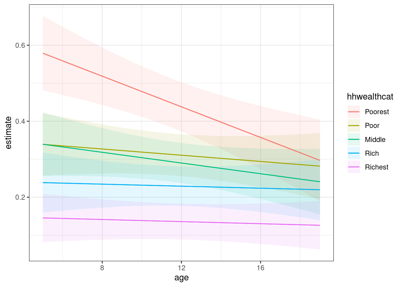
Interaction terms allow you to test whether the effect of one variable differs across subgroups — for example, whether the effect of age on walking to school differs across households of different wealth status. Interactions are easier to interpret on the probability scale, using the LPM or marginal effects/predictions.
Here is a quick example with the logistic model, suggesting that the effect of children’s age on the probability to walk to school matters mostly among the poorest households.
library(marginaleffects)m4 <-svyglm(walk ~ sex + age + edu_parent + hhwealthcat + province + age:hhwealthcat,design = design_edu)plot_predictions(m4, condition =c("age","hhwealthcat"))+theme_bw()
11.8 Exercise
After discretizing age, and adding sector (rural, urban, estate) as a new independent variable among geographical predictors, re-estimate the LPM and logistic models. Compare the results and interpret.
Children who go to school by bus are coded as 6 in the variable transport_medium. How does the probability of going to school by bus vary according to socioeconomic and geographical markers?
For your own group project, estimate logistic regressions. How do the results confirm/enhance your previous bivariate analyses?