install.packages("tidyverse")
library(tidyverse)1 Introduction
1.1 Install R and RStudio
First, you need to install R according to your computer’s configuration, using the links available on the Comprenhensive R Archive Network (CRAN).
Then, you can install RStudio by going to this page. RStudio is an “Integrated Development Environment (IDE)”, that is a software that provides a user-friendly interface for working with the R programming language. Note that it is possible to use other interface software, but RStudio is probably the most widely used today, and the one we will use during this training.
If, for one reason or another, it is not possible to install R or/and RStudio on your computer, you can temporarily use R / RStudio online by creating an account on the “Posit cloud”. However, we do not recommend this option for a long-term use as sensitive data should be stored on secured and personal servers.
Once R and RStudio are installed on your computer, you can directly open RStudio. It displays a nice console. You can create your first R script by clicking on the small white arrow on a green background and save it under the name 1Intro.R.
1.2 R, RStudio and the tidyverse
R is a programming language developed since the 1990s. It is derived from the S language and also shares some similarities with the C language. It is open-source and free of charge.
Among the many strengths of R, it has a large community of users, who can also take on the role of developers who continuously contribute to improve R language and what it can do. R therefore has numerous extensions in the form of functions, stored in packages (or libraries), which greatly facilitate its use. The list of packages available on CRAN is available here: https://cran.r-project.org/web/packages/. Although we will not be using them in this training seminar, please note that it is also possible to use packages that are not on CRAN.
With more than 22,000 packages, it’s easy to get lost. Throughout this guide, we will review a few packages that we considered helpful for making life easier when doing statistics in the social sciences. Again, let’s underline here that the goal of this guide is not to be exhaustive, nor to impose anything. One particularity of R is that it is often possible to do the same thing using different operations / functions / packages. Everyone eventually finds their own little “tricks”!
The tidyverse package includes a suite of packages designed to work together, making data manipulation, recoding, and the production of graphics easier compared to the basic R language, often referred to as “base R”. We will rely on functions and tools from the tidyverse package for our statistical work. You can have a look to the following small presentation of the tidyverse.
Note
You only need to install packages once; however, you must load the package each time you open a new R session. So, if you close RStudio and then reopen it, there is no need to run install.packages("tidyverse") again — but to use the functions from this package, you still need to load the tidyverse package by running the following code: library(tidyverse).
Calling the relevant packages is generally done systematically at the beginning of the script.
1.3 RStudio as a working tool
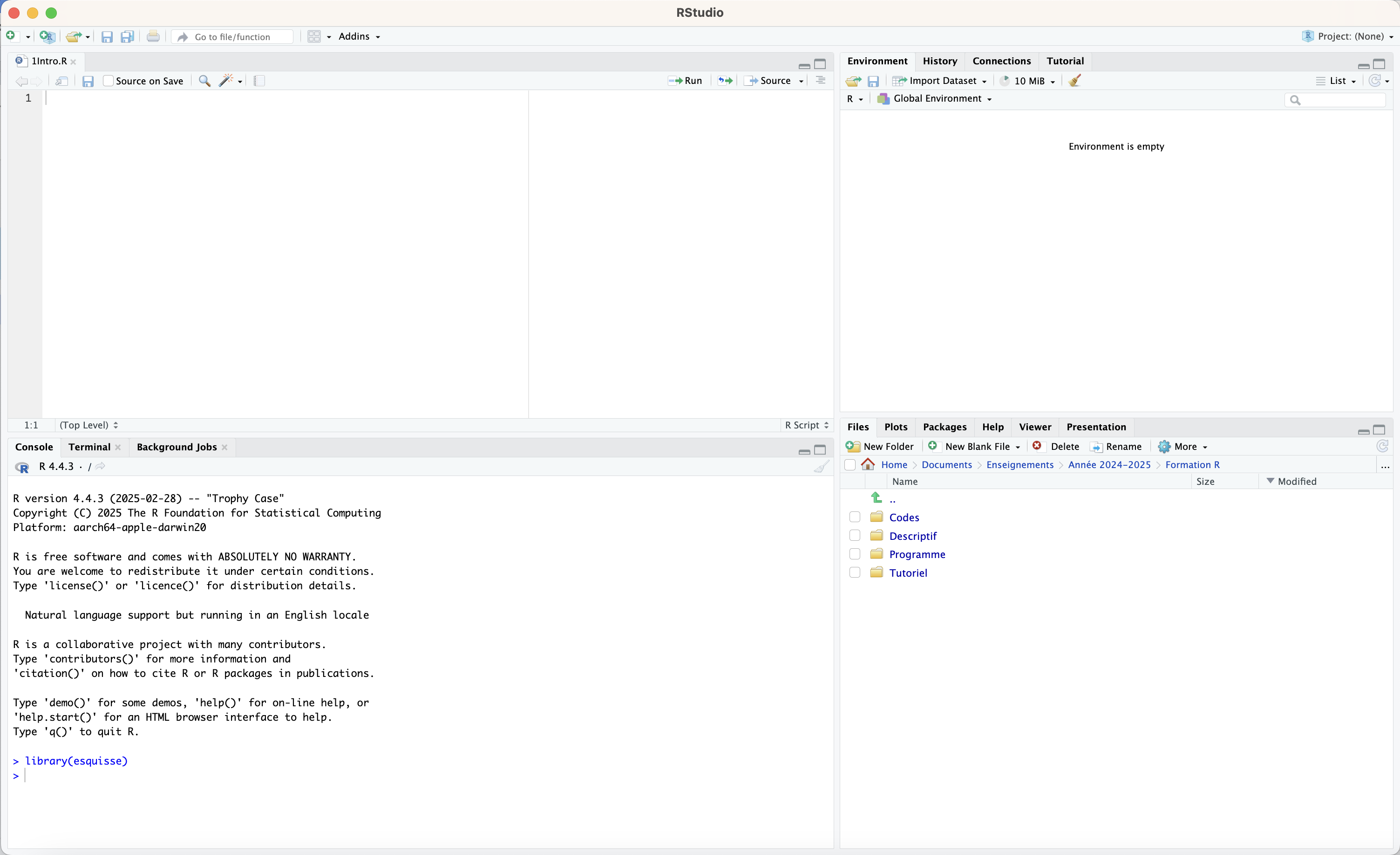
By default, the console is displayed in the form of four panels:
The first panel in the top left corresponds to the R script file, which for now is empty (or almost empty, if you have already copy-pasted the lines of code to install and load tidyverse). This is where we will write the command lines that we will run, either by clicking the ‘Run’ button, or by using the keyboard shortcut Cmd + Enter (or Control + Enter).
The second panel in the bottom left corresponds to the console. For now, it simply tells us that it has loaded R in the most up-to-date version found on my computer (4.4.3). The console will display the commands that we have run and the messages returned by R when executing them.
The third panel in the top right contains several tabs. The most important one is the Environment tab, which shows all the objects created in the current session (data frames, lists, vectors, etc.).
The fourth panel in the bottom right also contains several tabs, including:
Files (which allows you to browse your computer’s directory structure),
Plots (where our beautiful graphs will be displayed),
Packages, which lists the packages (libraries) installed on our computer and indicates which ones are loaded in the current session (they are checked),
Help, which displays information about a function when you type
?function_namein the console,and Viewer, where our nice tables will appear.
Caution
When quitting RStudio, a window may appear asking whether you want to “Save the workspace image…”. Warning: in fact, it is not a good idea to click Save!
Because this saves the entire workspace (the session), which will be automatically reopened when restarting RStudio, and you may end up with objects (for example, old databases that you used for former projects) that are no longer relevant for a later session (and that may even conflict with one another).
If you did not click on ‘Save’, reopening RStudio resets the R session. To make sure this is really the case (clear the global environment, unload packages, reset memory, etc.), you can type the following code in the console:
.rs.restartR()1.4 Loading data into R
To do statistics, we need data. Here, we are going to use excerpts of the Household Income and Expenditure Survey 2019 collected by the Sri Lankan Department of Census and Statistics.
The full questionnaire of the survey is shown below. We will mainly use Sections 1, 2, 3A, 3B, 7, and 8 of the questionnaire.
For legality matters, you will need to create an account on the Lanka data platform and download the microdata files from the online platform. Notice that you are able to download only 25% of the total survey sample.
For this workshop, we have additionally prepared four files to make your life easier to manipulate the survey, which you can access here Data repository. You will need to provide a password (request password by email!). Download the files from this online folder. The folder contains a PDF of the questionnaire and a zipped folder which you can unzip on your computer. In the zipped folder, you will find four “.rds” files (R statistical files):
demo.rdscontains data from Section 1 of the survey, i.e. on demographic characteristics of all household membersedu.rdscontains data from Section 2 of the survey, i.e. on school education for household members aged 5 to 19health.rdscontains data from Section 3A of the survey, i.e. on health treatment and chronic illnessenvironment.rdscontains data from Section 7 & 8, i.e. on access to primary facilities and housing information
WARNING: The unit of analysis (a “row” in the data file) differs in the four different files. For demo.rds, a row in the data file refers to one household member, irrespective of their age (N=19,848). Within a household, each member has its own row. For edu.rds, one row also refers to one individual from a household, but this time there is an additional age restriction: only household individuals aged 5 to 19 (N=4,552). For health.rds , one row refers to one individual; even if there is no age restriction, the sample is smaller than demo.rds since some individuals did not answer questions related to health in the questionnaire (section 3A) (N=18,468). Finally, for environment.rds, one row refers to one household (and not to one individual, as it is the case in the other datasets) (N=4,982).
In addition to the variables (the different “columns” of the files) specific to each file, we have already added a number of socio-demographic variables in the files with data at the individual level (demo.rds, edu.rds and health.rds) to ease statistical manipulations, including:
hhid: a unique household identifier (also available inenvironment.rds)indid: a unique individual identifieredu_attained: this is a recoded version of individual educational attainmentedu_father: father’s educational attainment (only inedu.rds)edu_mother: mother’s educational attainment (only inedu.rds)edu_parent: combined parents’ educational attainment, i.e. maximum educational attainment between both parents (only inedu.rds)age: individual’s agebirth_year: individual’s year of birthsex: individual’s sexage_father: father’s age (only inedu.rds)age_mother: mother’s age (only inedu.rds)province: province of residenceethnicity: household head’s ethnicityreligion: household head’s religionhhwealth: a continuous variable to proxy households’ material well-being (an index based on durable goods ownership which we constructed ourselves)hhwealthcat: a categorical variable to proxy households’ material well-being (an index based on durable goods ownership which we constructed ourselves)finalweight_25per: a “survey weight” variable to use in all statistical treatments to get correct estimates!
Let’s load edu.rds into RStudio. Generally, there are three options to import data into R:
In the bottom-right panel, you can browse your folder structure to find the appropriate file, and click on it.
You can click Import Dataset in the top-right panel, then click Browse and navigate through Finder or File Explorer.
You can directly use lines of code written in your script to load your file.
The third solution is preferable, in the interest of making your code reproducible. But the first or the second have the advantage of being easier when you are not familiar with coding, especially since these “point-and-click” solutions also provide the corresponding lines of code, which you can copy into your script for your next working session!
#Adjust the working directory with the path where your data are stored on your computer
setwd("/home/groups/3genquanti/SoMix/HIES for workshop")
edu<-readRDS("edu.rds")
1.5 Describe your dataset
The dataset should now appear in the Environment (top-right tab).
To see the data file (you can also click on it):
View(edu)Several ways of better describing your dataset can be useful:
You can type the name of the dataset
eduin the console, which will display the dataset: we do not recommended this option!You can also type
str(edu)to understand the structure of the dataset.You can also type
summary(edu)to obtain a summary of the quantitative variables in the dataset.
1.6 A few functions to manipulate data
1.6.1 Accessing a variable
The dataset is therefore composed of 38 variables. To access a variable — for example the variable age — you can type:
edu$ageThe $ sign indicates that we are accessing the variable age contained in the edu dataset. This command returns a vector of the values of the variable.
In the tidyverse, we call objects using pipes, which come in two different (and largely equivalent) operators: %>% and |>. We will favor the second one (but they are largely interchangeable!).
For example, to calculate the mean of age, we would write:
edu |> summarise(mean(age))summarise is the function that allows you to summarise the dataset according to the function specified. Note that we could also have written:
edu |> summarise(Mean_age=mean(age))
edu |> summarise(`Mean age`=mean(age))
1.6.2 Transforming a variable
Let’s assume the database does not include age but only year of birth (birth_year). In that case, we could create a variable returning individuals’ age using the information from the variable birth_year. Here, we use the function mutate to create/transform variables. Since the data that we use have been collected in 2019, we can then create a new variable that we decide to name ‘age_created’ to return individual’s age using the following code:
edu <- edu |> mutate(age_created=2019-birth_year)1.6.3 Selecting columns
To create a database called edu2 where we select only certain variables from the initial database edu, we write:
edu2<- edu |> select(hhid,age,sex,edu_attained)select allows to select only some columns (that is, some variables, as one column refers to one variable) of the dataframe.
Similarly, select can be used to remove columns:
edu3 <- edu2 |> select(-c(edu_attained,sex))1.6.4 Selecting rows
To create a database from edu where we decide to study only male respondents:
edum <- edu |> filter(sex=="Male")filter allows you to select the rows of the dataset that satisfy a given condition (in this example, we keep only the rows for which the variable sex equals the modality “Male”; in other words, we keep only male respondents). The ampersand operator & means “and”. If you want to use the logical “or” operator, you write: |.
Let’s say we want to study only female respondents with less than primary attainment:
edufl<- edu |> filter(sex=="Female" & edu_attainment=="Less than primary")1.6.5 Renaming a variable
Let’s rename a variable in edufl:
edufl <- edufl |> rename(ethnic_category=ethnicity)The variable ethnicity has been renamed as ethnic_category.
1.7 Saving data
To save databases from R (because you have done some data management and want to save your file), there are several solutions.
1.7.1 Native R formats
- You can save your data in .RData format. This is the simplest option — no hassle — and the advantage is that you are sure to preserve the format of the variables, the labels (we will come back to this later), etc.
save(edufl,file="edufl.RData")Before using this function, we should not forget to run setwd("path to the folder where we want the file to be saved") to indicate where to save the file (or at least to check that R is indeed pointing to the desired folder using the getwd() command).
Note that the RData format can perfectly well be used to save several R objects in the same file:
save(edufl,edum,file="eduv2.RData")To reopen an .RData file, you simply need to write:
load("eduv2.RData")The drawback of the .RData format is that, since there may be several objects in the file, we do not know what they are called and we cannot directly assign a default object name when opening it in the R console. This can sometimes be risky (imagine that we have a file eduv2.RData that contains edufl and edum, but that we already have an object called edum in our environment that is actually different — when opening eduv2.RData, the existing object would be overwritten).
For this reason, datasets can be saved individually using the .rds format with specific functions (this is how you have been provided with the workshop data):
saveRDS(edum, "edum.rds")When opening an .rds file, you explicitly control the name that will be assigned to it in the R environment (which in this case does not necessarily need to be edum):
edum2 <- readRDS("edum.rds")1.7.2 CSV format
- We sometimes need to export our data in CSV format. In that case, we use functions from the readr package, such as
write_csv(which uses commas as column separators and periods as decimal markers).
The CSV format with comma separators is the international standard for CSV files, and it is easily formatted when Excel on one’s computer is configured in English:
write_csv(edu, "edu.csv")1.7.3 Other formats
- If you want to save your file directly as an Excel file, this is also possible. At least two packages allow this: writexl and openxlsx. If we install openxlsx (
install.packages("openxlsx")):
library(openxlsx)
write.xlsx(edu, "edu.xlsx")
If you want to read an Excel file, you can use read.xlsx from the same package. Here, the argument sheet=NULL indicates that we are reading all the sheets of the Excel file if there are several:
read.xlsx("Salaires.xlsx", sheet = NULL)- Sometimes we work with colleagues who use other proprietary paid softwares (what an idea!). In that case, we can use the haven package, which allows to save data in SAS, SPSS or Stata format:
library(haven)
write_dta(edu, "edu.dta")
write_sas(edu, "edu.sas7bdat")
write_sav(edu, "edu.sav")
Be careful: with the SAS format, the conversion of value labels is not as straightforward as with other software.